Until now the oscilloscope quietly sampled at the display's pace, about 60 samples per second, which aliased anything faster than a slow blink into fiction. A 490 Hz PWM wave and a 555 running at audio rate looked like garbage because, at that sample rate, they were. This release moves acquisition inside the solver and adds the numbers a scope is supposed to give you.

Sampling that keeps up

Scope and logic samples are now captured inside the simulation loop itself, on a grid of up to 10,000 samples per second depending on your time window. The instrument reports its effective sample rate and the Nyquist frequency it implies, counts only real solver output as valid, and shows explicit gaps where acquisition paused rather than inventing a line across them. Freezing the display inserts a clean gap; a momentary button press no longer wipes the trace and redraws from the left.

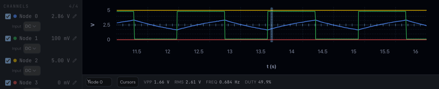
Measurements and cursors

Turn on Measurements in the scope's display menu and a strip under the plot reads Vpp, true RMS, frequency, and duty cycle for a chosen channel. The estimators are honest: amplitude statistics use every valid displayed sample, timing statistics use the longest gap-free stretch, and when there are not enough cycles in the window to be sure, the readout says Unavailable instead of guessing. On the 555 blinker above, the strip reads 0.684 Hz against the 0.686 Hz the datasheet formula predicts, which is the kind of agreement you want from a teaching instrument.

Cursors live in the same strip: two draggable time markers with Δt, 1/Δt, and ΔV readouts, keyboard operable, in colours that never collide with the eight node colours. Pause first for precise placement.

Noise you can trust, coupling you can choose

The old display noise was cosmetic fuzz scaled to your zoom level, which meant changing the vertical range changed the apparent noise voltage. It is replaced by an optional, deterministic front-end noise model with a declared density and bandwidth, off by default, and excluded from measurements, cursors, and captures. Each channel also gains DC or AC input coupling and a declared 12-bit ADC quantisation model with a stated input span, so the plotted trace is an instrument's view of the node, stated as such.

The meter comes to the simulator

The two-probe multimeter, previously a Learn exclusive, is now in the simulator: drag the red and black tips to pins or holes, read voltage, resistance, or a branch current, with HOLD to freeze the display. It is labelled an ideal observer, because it is one: no probe loading, no burden voltage. Learn's own multimeter was redesigned as a handheld smart DMM in the same release.

Fixes and improvements

• The toolbar status pill explains itself in plain language: healthy, settling, slow, straining, or error, each with one sentence about what to do.
• Numeric acquisition and model disclosures are tucked behind a "Show engine diagnostics" setting, keeping the scope graph-first by default.
• Logic analyzer thresholds follow the receiving chip's real logic family; mixed families ask for a manual threshold instead of picking one arbitrarily.

The full acquisition contract, including exactly what the sample grid and the effective-rate numbers mean, is written down at docs.devoltapp.com/user/oscilloscope-and-analysis.